The Power and Potential of Ray

Ray is a general purpose distributed computing paradigm that has been gaining momentum in both open source and commercial circles.

People are using it for a wide variety of tasks: from a substrate for other distributed systems like Horovod, as customers of some high quality libraries written on Ray such as Tune for hyperparameter optimization, and as part of third party libraries.

But one thing that these uses don’t reveal is the power and potential of Ray to make distributed computing dynamic and less rigid, and just how easy it is to parallelize existing code compared to prior techniques. This — for me — is the power and potential of Ray and the offshoots and imitations that will succeed it.

What I’d like to share with you in the next few sections is an example of code that was difficult to parallelize, but which Ray makes easy to parallelize. Two relatively straightforward refactors led to to a 60% improvement in performance on my local machine, and a 15x performance improvement in the cloud.

I recently learned this out on a problem that hasn’t been so easily amenable to distributed computing. I chose to explore decision trees and parallelizing them. There is some prior work here (such as this), but what I want folks to consider is the complexity of the approach to parallelization.

While they’ve fallen out of fashion in the age of deep learning, decision trees do have advantages: you don’t need a lot of data to train them, they can execute super quickly since they’re basically nested if-then statements, and they only have a few hyperparameters/architectural choices. Most importantly for this discussion, as Joachim Valente demonstrates (well worth reading if you’d like to understand decision trees),you can implement a simple decision tree building algorithm in under 70 lines.

You’d be surprised where decision trees end up — they might end up doing body segmentation on a depth camera, or ranking Airbnb experiences.

So I took Joachim Valente’s code and asked: if I wanted to parallelize it using Ray, what would it take? I had previously struggled with this in both my PhD twenty years ago, and as we were preparing to launch indoor location ten years ago at Google. People had parallelized around decision trees with things like random forests and bagging, but not much work had been done about building individual decision trees.

Existing parallelization models like Hadoop were just not flexible enough to tackle the recursive and dynamic parallelization challenges with decision trees. At the other end, models like posix threads didn’t scale beyond a single machine and message passing/RPCs were exceedingly complex.

Here’s what it took to Rayify decision tree building, and how relatively simple refactorings can lead to big performance improvements.

Step 0: Environment and imports

We start with a base version of the code available in this branch.

You can set up ray and the libraries we’ll use with a simple pip command:

% pip install ray numpy pandas sklearn

Next we need to add a few more imports and an init to cart.py. We’re also going to rip out the main function and use a different dataset that will allow us to explore more what it’s like to train with larger data — the forest covertype dataset. It has 580,000 examples, and 54 dimensions.

import ray
import pandas as pd
from sklearn import datasets, metrics
import time
import tree
...
if __name__ == "__main__":
  ray.init()
  dataset = datasets.fetch_covtype()
  X, y = dataset.data, dataset.target - 1 # 1-7 --> 0-6
  training_size = 100000 # only use first 100,000 for training
  max_depth = 8
  clf = DecisionTreeClassifier(max_depth=max_depth) 
  start = time.time()
  clf.fit(X[:training_size], y[:training_size])
  end = time.time()
  print("Serial execution took", end-start)
  y_pred = clf.predict(X[training_size:])
  print(metrics.classification_report(y[training_size:], y_pred))

Executing this produces the following output:

Tree building took 421.71840476989746 seconds
Test accuracy: 0.5620254796138142

Hmm … 7 minutes is OK. The accuracy is not great at 56%, but that’s a discussion for another article: for now, we’ll just be using the accuracy to verify that our parallelized versions don’t give different results.

Now that we have the basic infrastructure set up, let’s move on to parallelizing them.

Step 1: Distribute tree growing

The way that decision trees work is that it is a recursive “divide and conquer” algorithm. It finds the “best” attribute and threshold (like “density < 5”) to split on, splits the data into two halves and then recursively builds each half of the tree.

Because of the split, the two trees are independent, and so they can be built in parallel.

Let’s look at a function for growing trees locally. First, we need to move the grow_tree method of the DecisionTreeClassifier class out to be a function. Ray allows us to parallelize functions as tasks, not methods— this is a little counterintuitive, but it’s a small price to pay. We pull out this method to become grow_tree_local, and aside from an s/self/tree/g; there’s not much else to do.

The key lines are 16 through 24: find the best way to split the data, into two subtrees left and right, and then repeat recursively for each of them.

Next is where the magic happens: we write a new version of grow_tree_local that starts to use the power of Ray. Let’s call it grow_tree_remote.

You’ll notice that this code is almost identical to the code for grow_tree_local. The only changes are:

• The @ray.remote annotation at the beginning.
• On line 24, we do a quick “is this worth doing potentially remotely” test. We check if either side of the tree is big. tree_limit is a class property we added with a value of 5000 for now, but we’ll talk about that shortly.
• If it’s smallish (lines 29–31), it calls grow_tree_local method we’ve already discussed.
• If it’s largeish (lines 25–28), it then creates two ray tasks: one for the right and one for the left. It then calls ray.get for each of them (which is a blocking call). Futures are used to represent the as-yet uncompleted tasks.

One last change we have to make is that we now need to redefine the class method so that it calls the remote version.

def _grow_tree(self, X, y, depth=0): 
  future = grow_tree_remote.remote(self, X, y, depth)
  return ray.get(future)

OK, it can’t be that easy, can it? Let’s run it.

Tree building took 256.2617537975311  seconds
Test Accuracy:  0.5620254796138142

With this minor refactoring and a 6 line change that’s conceptually simple, we’re now running way faster — about 40% faster on our local machine. It’s taking advantage of all those extra cores to do something useful. Not bad for 20 minutes of work.

If you’d like to see the changes we made, here’s a comparison.

Step 3: Optimizing finding the best split

As we saw above, the decision tree proceeds by finding the best split in the data, splitting the data and recursing. We’ve now optimized the “recursing” part, but finding the best split is still done serially across the attributes. At the root node, for example, we are considering hundreds of potential splits across more than 50 attributes with hundreds of thousands of examples.

Can we parallelize this as well? The good news is that if we can pull this off it is almost complementary to the recursive optimization above. Parallelizing the search for the best split really helps at the root node, while parallelizing the tree building helps more as we split the tree building first into two tasks, then four tasks, then 8 tasks — that’s the point where it starts to kick in.

This turns out to be slightly more complicated to do, but still not very hard.

Let’s begin as before by starting with the “best split” function.

This iterates over every index and finds the best split point for that index. In order to parallelize this, we first need to refactor out the index part. We do this by adding a new method best_split_for_idx . You’ll see that we take the loop over attributes and turn that loop into a function.

We also wrap the best_split_for_idx in a remote ray version.

Now we go back and use these two new functions to rewrite our best split function.

You’ll see that the inner loop in best_split has been replaced by list comprehension, followed by code that finds the index and threshold of the smallest value. As before, there’s a feature_limit that we use to decide about whether it’s worth parallelizing or not.

Finally, we now need to make a small modification to our class method to use this version instead.

def _best_split(self, X, y):
  return best_split(self, X, y)

Let’s try running this again.

% python cart.py
Tree building took 171.66774106025696  seconds
Test Accuracy:  0.5620254796138142

So collectively, these two optimizations have reduced the computation time by a whopping 60% (from 420 seconds to 170 seconds). And I still haven’t left my laptop. One hint that it is really parallel is that my fan starts to come on really loudly while for the first serial case it barely broke a sweat.

If you’d like to see the changes we made for this step, you can see them here.

Step 4: The Cloud

One of the beauties of Ray is now that this is running on your laptop, you need to do very little to run it in the cloud. While setting up the cluster is beyond the scope of this article, suffice it to say it didn’t take long to set up a cluster of 4 machines (e2-standard-8’s, 8 vCPUs and 32GB each) on Google Cloud Platform.

To run this requires a small modification to the script:

ray.init(address='auto')

and that’s about it.

Here’s the non-parallel version result:

Tree building took 992.2957256235925  seconds
Test Accuracy:  0.562025479613814

And here’s the parallel:

Tree building took 64.12700819969177  seconds
Test Accuracy:  0.562025479613814

So now, we see that running on 32 cores across 4 machines, we get something like a 15x speedup, from 990 seconds on a single CPU, to 64 seconds on our little cluster.

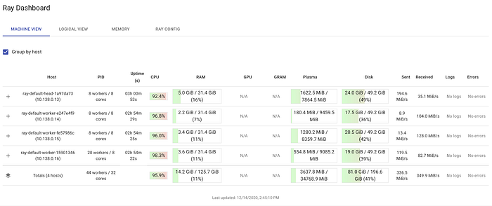
As you can see from the dashboard, at times all 32 CPU are working on our little problem.

Wait, what about those magic numbers?

You’ll notice in the above that we had two magic numbers: the minimum size for building trees remotely and the minimum size for splitting nodes. How did we get these numbers?

We guessed them based on previous values. But the good news is the algorithm isn’t particularly sensitive to the choices of those numbers. Here’s a 3D plot that shows time taken vs the feature and tree limits.

The feature limits are on the x axis (500 to 2500), the tree limits are on the y axis (1000 to 6000) and the time taken to train is on the z axis. As you can see from the valley down the middle, it’s not super sensitive — any value around 1000 to 3000 for the feature limit, and 2000 to 6000 for the tree limit works.

What’s next?

We could do more to make this even better. We could parallelize the predict() method too with very little difficulty.

And the above is “copy heavy” — it makes a new copy of the data every time we build a node. We could look into using some of Ray’s shared memory capabilities to make it even faster (and probably more efficient — those copies take a significant amount of time).

Also, we have only really used one of Ray’s two key abstractions: the task. We could explore doing more with the Actor abstraction.

Finally, if we were interested in optimizing it further, we might spend some time working out good values for the feature limit and tree limits, instead of our crude grid search. Fortunately, there’s also a Ray library for that!

Conclusions

We took a simple machine learning algorithm that has historically been hard to parallelize. We showed two simple refactors that led to a 60% improvement on a laptop. Those refactors show the power of Ray for dynamic and yet simple parallelism mechanisms. We showed that exactly the same code can run in the cloud with a 15x speedup.

Ray is an example of one such system, but what we are seeing is that distributed computing — and with it a way to sidestep the limitations of Moore’s law — is becoming more flexible, dynamic and yet simpler. This is why I’m excited about the power and potential of Ray and other advances in distributed computing.